Microsoft Excel is a powerful and popular spreadsheet program used by businesses and individuals worldwide. One of the essential skills to master when using Excel is moving around the worksheet quickly and efficiently. In this article, we will explore various ways to navigate around an Excel worksheet and discuss some default settings that can be customized to streamline your workflow.

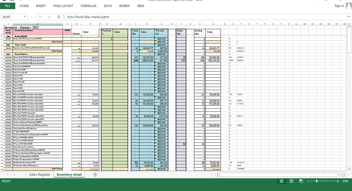
Excel worksheets are made up of both rows and columns. Rows are numbered 1 through 1,048,576 and run horizontally across the worksheet, while columns are labeled A through XFD and run vertically. The column labeling system in Excel follows a specific pattern. After column Z comes column AA, which is followed by AB, AC, and so on. After column AZ comes column BA, BB, BC, and so on. Similarly, after column ZZ, the columns are labeled AAA, AAB, AAC, and so forth. This system allows for a large number of columns to be included in a single worksheet.

In Excel, a cell is formed at the intersection of a row and a column, and each cell has a unique address that is determined by its column letter and row number. For instance, the upper-left cell of a worksheet is represented by the address A1, while the cell at the lower right corner of the worksheet is identified as XFD1048576. This address system makes it easier for users to locate and reference specific cells within the worksheet.

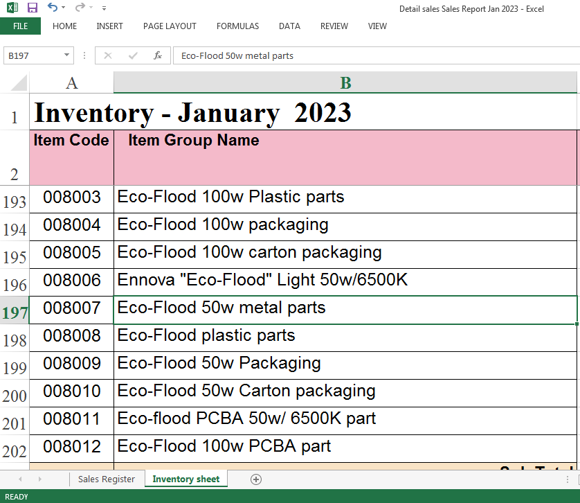
In Excel, there is always one cell that is considered the active cell, which is the cell that currently accepts keyboard input and can be edited. The active cell is typically indicated by a darker border around it, as shown in Figure 1.2. If you have selected more than one cell, the dark border will surround the entire selection, and the active cell will be the light-colored cell within the border. You can also identify the active cell by looking at the Name box, where its address will be displayed. However, depending on the method you use to navigate through your workbook, the active cell may or may not change.

The active cell is the one with the dark border—in this case, cell B197.

In this article, we will discuss:

1. Introduction
2. The Basics of Moving Around an Excel Worksheet
   • Using Arrow Keys
   • Using the Mouse
   • Using the Keyboard Shortcuts
   • Using the Scroll Bars
3. Customizing the Scroll Bars
4. Customizing Default Settings
   • Changing the Default Font
   • Adjusting Default Worksheet Size
   • Changing Default Workbook View

1. Introduction: Moving Around an Excel Worksheet

Excel is a powerful tool for organizing and analyzing data, but it can be overwhelming for new users. One of the most fundamental skills to learn when using Excel is how to navigate around the worksheet efficiently. In this article, we will explore the basics of moving around an Excel worksheet and discuss some default settings that can be customized to streamline your workflow.

2. The Basics of Moving Around an Excel Worksheet

Using Arrow Keys

The simplest way to move around an Excel worksheet is to use the arrow keys on your keyboard. The up and down arrow keys will move you up and down one row at a time, while the left and right arrow keys will move you left and right one column at a time. If you need to move quickly to the end of a row or column, you can use the “End” key followed by the arrow key in the direction you want to go.

Using the Mouse

You can also use the mouse to move around an Excel worksheet. You can click on a cell and drag the mouse to select a range of cells, or you can use the scroll wheel to move up and down or left and right through the worksheet. To move to a specific cell, click on it with the mouse.

Using Keyboard Shortcuts

Excel has a variety of keyboard shortcuts that can help you move around the worksheet quickly. For example, pressing “Ctrl+Home” will take you to the top-left cell of the worksheet, while pressing “Ctrl+End” will take you to the last cell with data in the worksheet. You can find a list of keyboard shortcuts in the Excel Help menu.

Using the Scroll Bars

The scroll bars on the right and bottom of the worksheet can also be used to move around. Clicking and dragging the vertical scroll bar will move you up and down, while clicking and dragging the horizontal scroll bar will move you left and right.

3. Customizing the Scroll Bars

Excel allows you to customize the scroll bars to make it easier to move around large worksheets. You can adjust the size of the scroll bar and change the number of rows or columns that are displayed at once. To customize the scroll bars, go to the “File” menu, select “Options,” and then click on “Advanced.” Scroll down to the “Display options for this workbook” section and adjust the settings as needed.

4. Customizing Default Settings

Excel has many default settings that can be customized to make your workflow more efficient. Here are a few examples:

Changing the Default Font

If you find yourself changing the font every time you create a new workbook, you can change the default font in Excel. Go to the “File” menu, select “Options,” and then click on “General.” Under the “Personalize your copy of Microsoft Office” section, you can select a new font and font size.

Adjusting Default Worksheet Size

Excel defaults to creating new worksheets with a certain number of rows and columns. If you frequently work with larger or smaller data sets, you can adjust the default worksheet size. Go to the “File” menu, select “Options,” and then click on “General.” Under the “When creating new workbooks” section, you can set the number of rows and columns that are included in each new worksheet.

Changing Default Workbook View

If you prefer to work in a specific view, such as Page Layout or Normal, you can change the default view for new workbooks. Go to the “File” menu, select “Options,” and then click on “General.” Under the “When creating new workbooks” section, you can select your preferred view.

Rows and Columns Defaults of MS Excel: Moving Around an Excel Worksheet

Microsoft Excel is a powerful spreadsheet software used by millions of users worldwide. It provides a great set of features that can help you organize, analyze, and present your data in an efficient manner. One of the fundamental concepts of Excel is the use of rows and columns to structure your data. In this article, we will explore the default settings of rows and columns in Excel, and how you can customize them to fit your needs.

When you open a new workbook in Excel, you are presented with a blank grid consisting of rows and columns. By default, Excel sets the row height to 15 points and the column width to 8.43 characters. However, these defaults may not always be suitable for your needs, depending on the type of data you are working with. In this article, we will discuss how to modify the default row height and column width, as well as how to customize individual rows and columns to fit your data.

In this section we will cover:

1. What are Rows and Columns in Excel?
2. Default Row Height and Column Width
3. Changing the Default Row Height and Column Width
4. Modifying Individual Rows and Columns
5. Autofitting Rows and Columns
6. Wrapping Text in Cells
7. Freezing Rows and Columns
8. Hiding Rows and Columns

What are Rows and Columns in Excel?

Rows and columns are the basic building blocks of a spreadsheet in Excel. Rows run horizontally across the sheet, while columns run vertically. Each row is identified by a number, while each column is identified by a letter. The intersection of a row and column is called a cell, which is where you can enter and manipulate data.

Default Row Height and Column Width

Excel has default settings for row height and column width, as mentioned earlier. The default row height is 15 points, which is equivalent to approximately 20 pixels. The default column width is 8.43 characters, which may not be sufficient to display all your data if you have long text or numbers.

Changing the Default Row Height and Column Width

If you find yourself frequently adjusting the row height and column width in your worksheets, you may want to change the default settings to better suit your needs. Here’s how you can do it:

1. Open Excel and create a new workbook.
2. Right-click on any row number or column letter and select “Row Height” or “Column Width”, respectively.
3. In the dialog box that appears, enter your desired height or width and click “OK”.
4. Close the workbook and save changes.

Modifying Individual Rows and Columns

Sometimes, you may need to customize the height or width of individual rows or columns to fit your data. Here’s how you can do it:

1. Select the row(s) or column(s) you want to modify by clicking on the row number or column letter.
2. Hover over the border between two rows or columns until the cursor changes to a double arrow.
3. Click and drag the border to adjust the height or width.
4. Release the mouse button when you’re satisfied with the size.

Autofitting Rows and Columns

Autofitting rows and columns is a quick way to adjust their size to fit the contents of the cells. Here’s how to autofit rows and columns in Excel:

Autofitting Rows

To autofit the height of a row, follow these steps:

1. Select the row(s) you want to autofit by clicking on the row number(s) on the left-hand side of the worksheet.
2. Right-click on the selected row(s) and select “Row Height” from the dropdown menu.
3. In the “Row Height” dialog box, click “OK” to accept the default height or enter a specific height.
4. Alternatively, double-click the border between the row number(s) to autofit the row height to the tallest cell in the selected row(s).

Autofitting Columns

To autofit the width of a column, follow these steps:

1. Select the column(s) you want to autofit by clicking on the column letter(s) at the top of the worksheet.
2. Right-click on the selected column(s) and select “Column Width” from the dropdown menu.
3. In the “Column Width” dialog box, click “OK” to accept the default width or enter a specific width.
4. Alternatively, double-click the border between the column letter(s) to autofit the column width to the widest cell in the selected column(s).

Autofitting Multiple Rows and Columns

To autofit the height or width of multiple rows or columns at once, select the rows or columns you want to autofit and follow the steps above.

Autofitting All Rows and Columns

To autofit all rows and columns in a worksheet, follow these steps:

1. Click on the “Select All” button at the top-left corner of the worksheet or press “Ctrl+A” on your keyboard to select all cells.
2. Right-click on any selected row or column and select “Row Height” or “Column Width” from the dropdown menu.
3. In the “Row Height” or “Column Width” dialog box, click “OK” to accept the default height or width.

Wrapping Text in Cells

When you enter text in a cell, it may extend beyond the visible boundaries of the cell. In this case, you can wrap the text to fit within the cell without adjusting the row height or column width. Here’s how:

1. Select the cell(s) you want to wrap text in.
2. Right-click and select “Format Cells”.
3. In the “Alignment” tab, check the box next to “Wrap text”.
4. Click “OK”.

Freezing Rows and Columns

If you have a large dataset that requires scrolling to view, you may want to keep certain rows or columns visible at all times. This can be achieved using the “freeze panes” feature. Here’s how:

1. Select the row below and/or the column to the right of the rows or columns you want to freeze.
2. Click on “View” in the ribbon.
3. Select “Freeze Panes” and choose “Freeze Panes” or “Freeze Top Row” or “Freeze First Column”.

Hiding Rows and Columns

In some cases, you may want to hide certain rows or columns in your worksheet without deleting them. Here’s how you can do it:

1. Select the row(s) or column(s) you want to hide by clicking on the row number or column letter.
2. Right-click and select “Hide”.
3. To unhide the row(s) or column(s), select the rows or columns on either side of the hidden area, right-click and select “Unhide”.

Conclusion: Moving Around an Excel Worksheet

In conclusion, moving around an Excel worksheet quickly and efficiently is a vital skill for anyone who works with data. Whether you prefer using the keyboard, mouse, or a combination of both, Excel provides many ways to navigate through your data. Additionally, customizing default settings such as the scroll bars, font, and worksheet size can help streamline your workflow and make your work in Excel more efficient. We have discussed the default settings for rows and columns in Excel, as well as how to customize them to fit your needs. We have covered how to change the default row height and column width, modify individual rows and columns, autofit rows and columns, wrap text in cells, freeze rows and columns, and hide rows and columns.

By customizing the rows and columns in your Excel worksheets, you can improve the readability and organization of your data, and save time and effort in the long run.

FAQs: Moving Around an Excel Worksheet

1. Can I change the default font for just one worksheet in Excel?

• Yes, you can change the font for an individual worksheet by selecting the cells you want to change, going to the “Home” tab, and selecting the desired font and size.

2. How do I move between worksheets in Excel?

• You can use the keyboard shortcut “Ctrl+Page Up” and “Ctrl+Page Down” to move between worksheets in an Excel workbook.

3. Can I customize the color of the Excel gridlines?

• Yes, you can customize the color of the gridlines by going to the “File” menu, selecting “Options,” and then clicking on “Advanced.” Under the “Display options for this worksheet” section, you can select a new color for the gridlines.

4. How do I zoom in or out in Excel?

• You can zoom in or out by using the keyboard shortcut “Ctrl+Plus” or “Ctrl+Minus.” Alternatively, you can use the zoom slider in the bottom-right corner of the Excel window.

5. Can I customize the Excel ribbon?

• Yes, you can customize the ribbon in Excel by right-clicking on it and selecting “Customize the Ribbon.” From there, you can add, remove, or rearrange commands to create a custom ribbon that suits your needs.

Other Questions:

1. How do I reset the default row height and column width in Excel? You can reset the default row height and column width by right-clicking on any row number or column letter and selecting “Row Height” or “Column Width”, respectively. In the dialog box that appears, click “Reset” and then “OK”.
2. Can I change the default font and size in Excel? Yes, you can change the default font and size in Excel by going to the “File” tab, selecting “Options”, and then selecting “General”. Under “Personalize your copy of Microsoft Office”, you can choose a new font and size.
3. How do I merge cells in Excel? To merge cells in Excel, select the cells you want to merge, right-click and select “Format Cells”. In the “Alignment” tab, check the box next to “Merge cells” and click “OK”.
4. How do I split cells in Excel? To split cells in Excel, select the cell(s) you want to split, right-click and select “Format Cells”. In the “Alignment” tab, uncheck the box next to “Merge cells” and click “OK”. You can then use the “Text to Columns” feature to split the cell contents into separate cells.
5. How can I filter my data in Excel? To filter your data in Excel, select the range of cells you want to filter, click on “Data” in the ribbon, and select “Filter”. You can then select the criteria you want to filter by, such as a specific value or range of values.
6. Can I undo autofitting rows and columns in Excel? Yes, you can undo autofitting rows and columns by selecting the rows or columns you want to adjust, right-clicking and selecting “Row Height” or “Column Width”, and entering a specific height or width.
7. How can I quickly autofit all rows and columns in Excel? To quickly autofit all rows and columns in Excel, click on the “Select All” button at the top-left corner of the worksheet or press “Ctrl+A” on your keyboard to select all cells, and then double-click the border between any row number or column letter.
8. Why do some cells not autofit when I adjust the row height or column width in Excel? If a cell contains a lot of text or a large amount of data, it may not autofit properly when you adjust the row height or column width. In this case, you may need to manually adjust the cell’s size or use the “Wrap text” feature to fit the text within the cell.
9. Can I autofit rows and columns in Excel automatically as I enter data? Yes, you can use the “Autofit” feature to automatically adjust the row height or column width as you enter data.
10. To enable this feature, go to “File” > “Options” > “Advanced” and scroll down to the “Editing Options” section. Check the box next to “Automatically adjust column width” or “Automatically adjust row height” as desired.
11. Can I autofit rows and columns in Excel on a printed worksheet? Yes, you can autofit rows and columns in Excel on a printed worksheet by adjusting the print settings. To do so, go to “File” > “Print” and click on the “Page Setup” button. In the “Page Setup” dialog box, select the “Page” tab and check the box next to “Fit to” under the “Scaling” section. Enter the number of pages wide and tall you want the worksheet to be and click “OK” to save the settings.